Macroeconomic Policy and the Coronavirus

(The post is also going to be cross-posted at Lars Christensen’s Market Monetarist blog.)

As the coronavirus spreads across the world, there is growing concern about the economic implications of the virus and what, if any, policy action is required of governments. Some have proposed traditional stimulus measures to counteract the virus while others have proposed more targeted measures. However, before one can offer policy solutions, one needs to diagnose the problem. In this post, I will outline what the potential economic consequences of the coronavirus are and the corresponding policy implications.

The Diagnosis

There are three main consequences of the coronavirus that we should be concerned about. The first is part of a flight to safety. In the face of uncertainty, people often sell risky assets, so that they can buy safe assets. People prefer to hold physical cash or put their money in an insured bank account rather than holding risky assets. What this does is create a greater demand for money. At the level of the individual, an increased demand for money is most easily accomplished by a reduction in spending. However, if money demand is rising in the aggregate (assuming there is no policy response), this reduction in spending is similar to a traffic jam. Sometimes, all it takes is for a few people to slam on the brakes and suddenly traffic is at a standstill. The widespread reduction in spending is analogous to the traffic jam in the sense that the economic activity can grind to a halt because of a significant reduction in spending.

The two other consequences of the coronavirus are related to planning and containment. Right now, in places like the United States, most people are continuing to work as usual. However, if the experience of other countries is any indication, this might not continue. Those who are infected will be expected to miss work, even if the virus is not a threat to their health. In addition, there might be forced quarantines on particular areas.

In the event of self-quarantine or forced public quarantine, consumers will need to have food and medicine since they cannot leave their home. Furthermore, firms will need to be able to pay for non-operating costs during a quarantine. This includes making debt payments. Firms who are currently cash-strapped and that are relying on cash flow to make debt payments might find themselves unable to make debt payments because of quarantines. This could result in default and bankruptcies, which exacerbate the problem through the implications on financial markets.

The Prescription

So what is to be done?

The first thing to do is for the Federal Reserve to commit to do whatever it takes to maintain stability in aggregate nominal spending. As David Beckworth and I have shown, nominal spending crashes are rare, but the common cause is monetary and such events are associated with severe recessions. The Federal Reserve should commit itself to lowering interest rates and engaging in quantitative easing to the extent necessary to prevent a decline in nominal spending. I have written about why this is important in theory and in practice. In addition, the Fed should be tracking properly measured monetary aggregates, which are released more frequently than data on nominal spending. I have shown in my own research that these monetary aggregates are useful in predicting inflation and nominal spending. The Fed is already failing at this. Inflation expectations have been plummeting and their response has been inadequate.

The Trump administration has suggested a temporary payroll tax cut. Some have criticized this idea, but these critics are missing the point. A payroll tax cut is something that would work if it is done immediately. The cut in payroll taxes would increase profits to firms and increase take-home pay of workers. This would allow firms to start retaining these additional earnings now in order to make debt payments and pay other non-operating costs in the event that they have to temporarily shut down. This would also allow workers to use this additional income to make purchases to stockpile food and medicine in the event of self-quarantine or a forced geographic quarantine. However, this needs to be done now and will not be as effective once things have started shutting down.

Another policy prescription is to do lump sum transfers of around $1000 per taxpayer. Normally, these are somewhat controversial as a consequence of Ricardian equivalence. Under Ricardian equivalence, a transfer to taxpayers that is paid for through debt creation just results in a net increase in savings which offsets the debt creation and therefore has no effect on economic activity. While there is some debate about the degree to which Ricardian equivalence holds, this debate is largely irrelevant here. These checks would allow people decide how to allocate the money for its best use in preparation for the possible consequences of the virus. For some, this might mean using it as extra savings. For others, this might be a way to purchase food and medicine in anticipation of the consequences. The objective here is not to boost real GDP per se, but rather to plug holes before they have a chance to leak.

Finally, the government should implement temporary and mandatory paid sick leave financed by the government. This will give people the peace of mind that they will not lose their income in the event that they have the virus or otherwise are unable to work because of the virus. The policy also has the added benefit of preventing the virus from spreading since people are not forced making the difficult choice between working sick or losing income.

Some Links

A couple of links to things I have been working on…

• My paper entitled, “The Riksbank, Emergency Finance, Policy Experimentation, and Sweden’s Reversal of Fortune” is now forthcoming at the Journal of Economic Behavior and Organization. The paper includes a lot of background on Swedish governance and fiscal capacity, as well as information about the early Swedish monetary system and the Riksbank. I argue that the constraints on the Riksbank left Sweden unable to use its central bank in the same way that Britain did during times of war. I also argue that policy experimentation at the Riksbank had a negative effect on economic activity. I really enjoyed working on this paper, so I hope that others find some value in it.
• I have also written a review of Saez and Zucman’s new book, The Triumph of Injustice: How the Rich Dodge Taxes and How to Make Them Pay.

On Drawing the Wrong Lessons from Theory: The Natural Rate of Unemployment

Economic theory is important. Theory provides discipline. Economists write down a set of assumptions and follow those assumptions to their logical conclusions. The validity of a particular theory is then tested against observed data. Modern economic theory is often mathematical, but theory comes in a variety of forms. Sometimes theory is used to develop and test specific empirical predictions. Other times, economic theory acts as a type of sophisticated thought experiment. These thought experiments generate broader empirical predictions. In fact, some of these sophisticated thought experiments contain important lessons for monetary policy.

In the late 1960s, Milton Friedman suggested that monetary policy was limited in its ability to influence the unemployment rate. Friedman argued this point by discussing the concept of a natural rate of unemployment. The idea is that there is some unemployment rate that would exist in the economy based on the fundamentals of the economy. If the unemployment rate is equal to the natural rate, the central bank cannot permanently reduce the unemployment rate. The only way in which the central bank can lower the unemployment rate is by producing higher than expected inflation. The temporary decline in real wages would lead to an increase in output and lower unemployment. Ultimately, real wages rise and employment returns to its original level.

The theory proposed by Friedman is very much in the thought experiment variety. If we accept the idea of a natural rate of unemployment pinned down by real factors, then nominal changes will not have any long-run effect on the unemployment rate. This conclusion is a version of what economists call the classical dichotomy – the idea that nominal variables only affect other nominal variables in the long-run and real factors determine resource allocation.

Subsequent economists explored this concept of the natural rate of unemployment. Finn Kydland and Ed Prescott developed a model to consider what would happen if a discretionary central bank had a lower target for the unemployment rate than the natural rate. What they found is that, in equilibrium, the unemployment rate would equal its natural rate, but the rate of inflation would be higher than if their target for the unemployment rate was equal to the natural rate.

This sort of sophisticated thought experiment contains important lessons for monetary policy. For example, what the model shows is that a preference for unemployment to be lower than its natural rate does not allow discretionary policymakers to achieve this lower rate in equilibrium. Instead, the economy will always end up at the natural rate. Discretion will only lead to higher inflation. The broad lesson is that rules-based policy is better than discretionary policy because a rule would avoid this tendency to try to manipulate the unemployment rate.

Friedman’s concept of a natural rate of unemployment was inspired by Knut Wicksell’s natural rate of interest. According to Wicksell, the natural rate of interest is pinned down by the marginal productivity of capital in the economy. When the market interest rate is below the natural rate, this leads to an expansion of money and credit and therefore inflation rises. When the market interest rate is above the natural rate, money and credit contract and inflation declines. Both of these concepts – the natural rate of unemployment and the natural rate of interest – continue to play a role in the way that policy is discussed and conducted.

While the sophisticated thought experiments that draw upon these concepts contain important lessons for policy, it is important to remember that they are thought experiments. In reality, there is no empirically observable natural rate of unemployment nor a natural rate of interest. These are theoretical concepts used to motivate the thought experiment.

Economists, however, seem to have drawn the wrong lesson from such thought experiments. Since policy is neutral when the market interest rate is equal to its natural rate or when the unemployment rate is equal to its natural rate, economists have sought to estimate these natural rates. This is a problem because these are theoretical constructs. Estimates of these natural rates cannot be compared to some observable counterpart to assess their goodness of fit. Estimation often requires the use of some sort of structural model. The extent to which the estimate is useful depends on the external validity of the model.

This is worrisome because references to the natural rate of unemployment or the natural rate of interest have become more common among policymakers. The Federal Reserve consistently refers to purported inflationary “pressures” that come from declining rates of unemployment (which, by the way, reverses the direction of causation described by Friedman).

Rather than judging the stance of monetary policy by the proximity of the unemployment rate or the interest rate to their respective natural rates, central banks should rely on an explicit target of a measureable macroeconomic variable that the central bank can directly influence with policy. With an explicit target, there is no need to estimate the natural rate of interest or natural rate of unemployment. For example, suppose the central bank targeted a five percent growth rate for nominal income in the economy. If nominal income growth is higher than five percent, this indicates that policy is too expansionary. If nominal income growth is below five percent, then monetary policy is too contractionary. When nominal income growth is approximately equal to its target, policy is neutral. There is no need to estimate any natural rate.

The Federal Reserve’s dual mandate of stable prices and maximum employment is partly to blame for the emphasis on the unemployment rate and attempts to estimate a natural rate. However, an explicit target would provide a sense of neutral monetary policy in a much more straightforward and easily observable way. In addition, achieving maximum employment need not require explicitly targeting the unemployment rate or some other measure of employment. The objective of the central bank should be to achieve nominal stability, such as the stability of the growth of nominal income. With nominal stability, relative prices will adjust to allocate resources to their most productive use. This is the main lesson of Friedman’s thought experiment. Attempts to estimate a natural rate of unemployment draw the wrong lesson. Such estimates are an unwelcome diversion pursued under the guise of being scientific.

On Exhaustible Resources, Part 2

Yesterday’s post on exhaustive resources has drawn a lot of ire from critics. Some have argued that I didn’t address the problem of economic growth. In short, the argument is that there are two sources of economic growth. The first is that increased efficiency of resources allows us to produce more stuff with the same amount of resources. The second is that because resources are more productive we tend to use more of them. Others have argued that algebra is irrelevant to the problem.

I’d like to address both of these concerns because they are wrong. First, let’s address the algebra issue. The model I presented in my previous post is an example of using formal economic theory to make a point that is apparently not obvious to people. If society has exhaustible resources, will markets completely deplete those resources and leave us with nothing? What the model shows is that this will not happen. It doesn’t happen because as the resource is depleted, the price of the resource rises thereby encouraging people to use less of it. (Correspondingly, if resources are near the point of depletion shouldn’t energy prices be a lot higher?) So attacking me for using algebra will get applause from a certain type of audience and “algebra doesn’t solve environmental calamity” makes a really good bumper sticker, but it is not a valid critique. The model is an exercise in maintaining consistent logic.

Now to the more substantive critique. This is the critique that growth not only comes from changes in productivity but that these changes in productivity lead to greater resource use. So let’s tackle this problem head-on using a modified version of the Solow Model.

Before going through the model let’s recall the crux of the debate:

• George Monbiot claimed that perpetual growth is not possible in a world of finite resources.
• I replied that perpetual growth comes from finding more efficient ways to use resources (the ability to produce the same amount of stuff with fewer resources).

Let’s imagine that there is an aggregate production function that is given as

where is output, is the quantity of exhaustible resources, is capital, is a parameter, is the productivity of energy use. So has the interpretation of “effective units of resources.” Now let’s assume that

where is the rate of resource extraction. Note here that I am assume no uncertainty. The amount of resources are known and declining with use.

Also, I will assume that

where is the growth rate of the productivity of energy use.

Finally, the law of motion of the capital stock is given as

where is the savings rate and is the depreciation rate on capital.

Define as effective units of resources and as capital per effective unit of resources. The corresponding law of motion for capital per effective unit of resources is given as

From this equation, there is a stable and unique steady state equilibrium for if . A sufficient condition for this to hold is .

Now, let . Note that this implies that in the steady state, . Thus, output per effective unit of resources should be constant in the steady state. This implies that the growth rate of output itself satisfies

It follows that in the steady state equilibrium, we can experience perpetual economic growth so long as the productivity of energy use rises by more than enough to offset the rate of resource extraction. Put differently, we can experience long-run economic growth even in a world of finite resources as long as we continue to use those resources more efficiently. Recall that Monbiot argued that it is impossible. I, on the other hand, argued that this is incorrect because growth is the result of being able to produce the same amount of stuff with fewer resources. This is precisely what I meant.

Of course, we might wonder if this is actually going on in reality. So let’s go to the data. We can measure the productivity of resource use by plotting GDP relative to energy consumption. The following figure is from the World Bank.

As one can see from the graph, there has been a considerable productivity increase in the use of energy over the last few decades. This is not the whole story since this graph only measure . One would need to compare this to to determine whether we are currently on a sustainable path. Nonetheless, the claim made by Monbiot was that perpetual growth is not possible in a world of finite resources. What I have shown is that this is wrong as a logical statement. Furthermore, my basic model in this post actually understates our ability for perpetual growth since I assumed that it is not possible to substitute from the exhaustible resource to either another exhaustible resource or to a renewable resource.

On Exhaustible Resources

Yesterday, George Monbiot wrote in the Guardian that the survival of capitalism relies on persistent economic growth and persistent economic growth is impossible in the long-run because there are finite resources in the world. In response, I made the following popular, but sarcastic tweet.

Economists: economic growth results from finding ways to produce the same amount of stuff with fewer resources.

You, an intellectual: economic growth requires infinite resources. https://t.co/5jtGW80mcf

— Josh Hendrickson (@RebelEconProf) September 23, 2019

The tweet was meant to be funny. The format itself is a meme. Nonetheless, it does drive home the point that the source of economic growth is finding more efficient uses of resources. With this being the internet, however, I started receiving replies telling me that I was an idiot who doesn’t understand exhaustible resources and even had one person recommend that I read up on resource economics. As it turns out, I know a little bit about resource economics — and wouldn’t you know it, resource economics actually supports my position. So I thought it was worth a blog post.

Let’s imagine that we have an exhaustible resource. Suppose that the quantity of the exhaustible resource at time is given by , where . Now let’s suppose that follows a geometric Brownian motion:

where is the rate of resource extraction, is the standard deviation, and is an increment of a Wiener process. The intuition of this assumption is as follows. First, zero is an absorbing barrier here. What I mean is that once , it is permanently there. This is the exhaustible resource part. Second, on average the amount of the resource that is available is declining by the consumption of the resource. Third, there is some uncertainty about the quantity of the resource that is actually available. For example, one might observe positive or negative shocks to the supply of the resource. In other words, there are times when new supplies of the resource are discovered. There are other times in which there is less supply than had been estimated. In addition, one could also include “technology shocks” as a source of positive movement in the supply of resources in the sense that better production processes tend to economize on the use of resources, which is basically the same thing as a discovery new amounts of the resource. In short, what we have here is a reasonable representation of how the supply of an exhaustible resource is changing over time.

Now suppose that the consumption of the resource gives us some utility, where utility has the usual properties. The objective is to maximize utility over an infinite horizon (with finite resources). Given the process followed by the resources, I can write the Bellman equation for a benevolent social planner as:

where is the rate of time preference (or the risk-free interest rate). The first-order condition is given as

Intuitively, what this says is that the marginal utility of the consumption of the resource is equal to the marginal value of the resource. Or that marginal benefit equals marginal cost. In fact, this implies that is the shadow price of the resource, or the spot price (more on this below).

Now, for simplicity, let’s suppose that consumers have the following utility function:

It is straightforward to show (after A LOT of algebra) that

So the rate of resource extraction is constant and a function of the parameters of the model. Or, if we assume that there is log-utility, we can simplify this to Let’s make this further simplification to economize on notation.

So we can re-write our geometric Brownian motion under log utility as

So now we have the evolution of resources in terms of exogenous parameters. We might be interested in the quantity of resources in existence at any particular point in time, say time . Fortunately, our stochastic differential equation has a solution of the form:

Since exponential functions are always positive and , it must be the case that .

So what does this mean in English?

What it means is that given the choice about how much to consume of a finite resource over an infinite horizon, the rate of resource exhaustion is chosen to maximize utility. Given the choice of consumption over time, the total supply of the resource will decline on average over time with the rate of resource exhaustion. However, the quantity of the resource will always be positive.

How is this possible?

Let’s return to the maximization condition:

Recall that I defined as the marginal value of the resource, or the shadow price of the resource. Note that as time goes by, is declining on average. Since is constant, when declines, the marginal utility of consumption rises because total consumption is declining. It must therefore be the case that shadow price of the resource increases as well. But the problem I described is a planner’s problem (i.e., how a benevolent social planner would allocate the resource given the preferences for society). Nonetheless, a perfectly competitive market for the resource would replicate the planner’s problem. What this means is that as the resource becomes more scarce, the spot price of the resource will rise so that people economize on the use of the resource. Consumption of the resource declines over time such that the resource is never completely exhausted.

Thus, and somewhat ironically given Monbiot’s point, it would be a deviation from competitive markets for the resource or poorly-defined property rights that might lead us to depart from this outcome. So it’s the markets that save us, not the people who want to save us from the markets.

A Simple Lesson About Money and Models

Imagine you are in your high school algebra class and you are presented with the following two equations:

Two linear equations with 2 unknowns. This is a simple problem to solve.

Now suppose that your teacher gives you the following three equations:

Note that this is still a simple problem to solve. The first two equations are identical to the previous example. You can use those first two equations to solve for x and y. Then, knowing x, you can solve for z. The central point is that the third equation is not important for determining the value of x. The first two equations are sufficient to solve for x and y.

So why am I bringing this up?

This is precisely how the benchmark New Keynesian model deals with money. The baseline New Keynesian model does not include money. The model is complete and a solution exists. Subsequently, to examine whether money would be important in the model, a money demand function is added to this system of equations. There is a solution to the model that exists. Money is then shown to be irrelevant in the determination of the other variables. But, then again, so was z.

UPDATE: I have updated the post to read “benchmark New Keynesian model” to reflect the fact that some have attempted to integrate money into the NK model in other ways, specifically through non-separable utility. This is, in fact, where I am going to take this argument in the future. Nonetheless, for now, see the excellent comment by Jonathan Benchimol below with some links to his related research.

How Did the Gold Standard Work? Part 1: The Efficiency of the Gold Standard

Sebastian Edwards has written an interesting new book about FDR’s devaluation of the dollar and the legal and economic consequences thereof. This post is not about the book, although I do recommend it. What I would like to write about is motivated by some of the reaction to this book that I’ve seen and heard regarding gold and the gold standard. In recent years, I have become convinced that what I thought was the conventional wisdom on the gold standard is not widely understood. So I’d like to write a series of posts on the gold standard and how it worked. My tentative plan is as follows:

Part 1. The efficiency of the gold standard.
Part 2. The determination of the price level under the gold standard.
Part 3. The Monetary Approach to the Balance of Payments vs. the Price-Specie Flow Mechanism
Part 4. Gold standard interpretations of the Great Depression.

I don’t have a timeline for when these will be posted, but it is my hope to have them posted in a timely fashion so that they can get the appropriate readership. With that being said, let’s get started with Part 1: The efficiency of the gold standard.

Some people define the gold standard in their own particular way. I want to use as broad of a definition as possible. So I will define the gold standard as any monetary system in which the unit of account (e.g. the dollar) is defined as a particular quantity of gold. This definition is broad enough to encapsulate a wide variety of monetary systems, including but not limited to free banking and the pre-war international gold standard. Given this definition, the crucial point is that when the unit of account is defined as a particular quantity of gold, this implies that gold has a particular price in terms of this unit of account. In other words, if the unit of account is the dollar, then all prices are quoted in terms of dollars. The price of gold is no different. However, since the dollar is defined as a particular quantity of gold, this implies that the price of gold is fixed. For example, if the dollar is defined as 1/20 of an ounce of gold, then the price of an ounce of gold is $20.

This type of characteristic poses a lot of questions. Does the market accept this price? Or, is there any tendency for the market price of gold to equal the official, or mint price? This is a question of efficiency. If the market price of gold differs substantially from the official price, then the gold standard cannot be thought of as efficient and one must consider the implications thereof for the monetary system. What determines the price level under this sort of system? Does the quantity theory of money hold? What about purchasing power parity? In many ways, these questions are central to understanding not only of how the gold standard worked, but also the nature of business cycles under a gold standard. The price level and purchasing power parity arguments are equilibrium-based arguments. This raises the question as to what mechanisms push us in the direction of equilibrium. We therefore need to compare and contrast the monetary approach to the balance of payments with the price-specie flow mechanism. Finally, given this understanding, I will use the answers of this question to gain some insight into the role of the gold standard with regards to the Great Depression.

In terms of efficiency, we can think about the efficiency of the gold market in one of two ways. We could consider the case in which the dollar is the only currency defined in terms of gold. In this case, the U.S. would have an official price of gold, but gold would be sold in international markets and the price of gold in terms of foreign currencies is entirely market-determined. Alternatively, we could consider the case of an international gold standard in which many foreign currencies are defined as a particular quantity of gold. For simplicity, I will use the latter assumption.

This first post is concerned with whether or not the gold standard was efficient. So let’s consider the conditions under which the gold standard could be considered efficient. We would say that the gold standard is efficient if there is (a) a tendency for the price of gold to return to its official price, and (b) if market price of gold doesn’t different too much from the official price.

Under the assumption that multiple countries define their currency in terms of the quantity of gold, let’s consider a two country example. Suppose that the U.S. defines the dollar as 1/20 of an ounce of gold and the U.K. defines the pound as 1/4 of an ounce of gold. It follows that the price of one ounce of gold is $20 in the U.S. and £4. Note that this implies that $20 should buy £4. Thus, the exchange rate should be $5 per pound. We can use this to discuss important results.

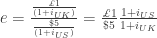
Suppose that the current exchange rate is equal to the official exchange rate. Suppose that I borrow 1 pound at an interest rate for one period and then exchange those pounds for dollars and invest those dollars in some financial instrument in the U.S. that pays me a guaranteed rate of for one period.

The cost of my borrowing when we reach the next period is . But remember, I exchanged pounds for dollars in the first period and 1 pound purchased 5 dollars and invested these dollars. So my payoff is . I will earn a profit if I sell the dollars I received from this payoff for pounds, pay off my loan, and have money left over. In other words, consider this from the point of view in period 1. In period 1, I’m borrowing and using my borrowed funds to buy dollars and invest those dollars. In period 2, I receive a payoff in terms of dollars that I sell for pounds to pay off my loan. If there are any pounds left over, then I have made an arbitrage profit. Let denote the forward exchange rate (the exchange rate in period 2), defined as pounds per dollar. It follows that I can write my potential profit in period 2 as

We typically assume that in equilibrium, there is no such thing as a perpetual money pump (i.e. we cannot earn a positive rate of return with certainty with an initial investment of zero). This implies that in equilibrium, this scheme is not profitable. Or,

Re-arranging we get:

This is the standard interest parity condition. Note that is defined as pounds per dollar. If the gold standard is efficient we would expect the forward exchange rate to equal to official exchange rate (we should rationally expect that the gold market tends toward equilibrium and the official prices hold). Thus, one should expect that . Plugging this into our no-arbitrage condition implies that:

In other words, the interest rate in both countries should be the same. There is a world interest rate that is determined in international markets.

However, remember that this is an equilibrium condition. Thus, at an point in time there is no guarantee that this condition holds. In fact, in our arbitrage condition, we assumed that there are no transaction costs associated with this sort of opportunity. In addition, under the gold standard, we do not have to exchange dollars for pounds or pounds for dollars. We can exchange dollar or pounds for gold and vice versa. Thus, under the gold standard what we really care about are market prices of the same asset in terms of dollars and pounds. For example, consider a bill of exchange. The price paid for a bill of exchange is the discounted value of the face value of the bill.

So if the ratio of the prices of these bills differ from the official exchange rate, there is a potential for arbitrage profits. As the equation above implies, this can be reflected in the ratio of interest rates. However, it can also simply be observed from the actual prices of the bills.

Officer (1986, p. 1068 – 1069) describes how this was done in practice (referencing import and export points as what we might call an absorbing barrier under which it made sense to engage in arbitrage, given the costs):

In historical fact, however, cable drafts in the pre-World War I period were dominated by demand (also called “sight”) bills as the exchange medium for gold arbitrage. Purchased at a dollar market price in New York, the bill would be redeemed at it pound face value on presentation to the British drawee, with the dollar-sterling exchange rate give by the market price/face value ratio. When this rate was greater than the (demand bill) gold export point, American arbitrageurs (or American agents of British arbitrageurs) would sell demand bills, use the dollars thereby obtained to purchase gold from the U.S. Treasury, ship the gold to London, sell it to the Bank of England, and use part of the proceeds to cover the bills on presentation, with the excess amount constituting profit.

[…]

When the demand bill exchange rate fell below the gold import point, the American arbitrageur would buy demand bills, ship them to Britain, present them to the drawees, use the proceeds to purchase gold from the Bank of England, ship the gold to the United States, and (if not purchased in the form of U.S. coin) convert it to dollars at the U.S. mint.

Thus, we can think of interest rate differentials as opportunities for arbitrage directly, or as reflecting the current market exchange rate. In either case, the potential opportunities for arbitrage profits ultimately kept gold near parity. In fact, Officer (1985, 1986) shows that gold market functioned efficiently (and in accordance with our definition of efficiency).

With this in mind, we have a couple of important questions. This discussion focuses entirely on the microeconomics of the gold standard. In subsequent posts, I will shift the discussion to macroeconomic topics.

The Phillips Curve and Identification Problems

Frequent readers of the blog (can you be frequent if I only write about 5 or 6 times a year?) will know that I often criticize the Phillips Curve. One counterargument that I receive to my complaints about the Phillips Curve is that my critiques are unfair because they ignore the role of countercyclical monetary policy. For example, suppose that the following two things are true:

1. The central bank responds to a positive output gap by tightening monetary policy.
2. Inflation is caused by positive output gaps.

If these two things are correct, the critics say, then you might fail to see an empirical relationship between inflation and the output gap (or even a negative relationship). However, this violates point (2) which we’ve assumed to be true. Thus, we have an identification problem. The failure to find an empirical relationship might be because countercyclical policy is masking the true underlying, structural relationship. (I could make a similar argument about the quantity theory that, for some odd reason, is not as popular as this story.)

Well, if identification is the problem, then I have a solution. During the period from 1745 to 1772, Sweden’s central bank, the Riksbank, issued an inconvertible paper money. What we would now call monetary policy was carried out through discretionary means. For example, the Hat Party, which controlled the Riksdag and the Riksbank from 1739 to 1765, expanded the bank’s balance sheet in an attempt to increase economic activity. However, while monetary policy was determined through discretion, there is no evidence whatsoever that the central bank used countercyclical policy. In fact, the Hat Party explicitly thought that monetary expansions would boost economic activity. The closest thing to a countercyclical policy occurred when the Cap Party took over and reduced the money supply in an attempt to bring down the price level. However, they did this so dramatically that any good advocate of the Phillips curve would believe that this would result in a negative output gap and deflation such that the relationship would still hold.

So, what we have here is a period of time in which the identification problem is not of any significance. As a result, we can have a horse race between the quantity theory of money and the Phillips Curve to see which is a better model of inflation.

Here is a figure from my recent working paper on the Riksbank that looks at the relationship between the supply of bank notes and the price level from 1745 – 1772. The solid line represents the best linear fit of the data. This graph seems entirely consistent with the quantity theory of money.

Now let’s look at a Phillips Curve for the same period. To do so, I construct an output gap as the percentage deviation of the natural log of real GDP per capita from its trend using the Christiano-Fitzgerald filter (the trend is computed using data from 1668 to 1772). Here is the scatterplot of the output gap and inflation.

Hmmm. There doesn’t seem to be any clear evidence of a Phillips Curve here. In fact, note that the relationship between the output gap and inflation should be positive. Yet, the best linear fit is negative (but not statistically significant). Maybe its the filter. Let’s replace the output gap with output growth (a proxy for the output gap) and see if this solves the problem.

Hmm. The Phillips Curve doesn’t seem to be there either. In fact, the slope is steeper (i.e., going in the wrong direction) and now statistically significant.

So here we have a period of time in which the central bank is using discretion to adjust the supply of bank notes and there is no role for countercyclical policy. The data is therefore immune to the sorts of identification problems we would see in the modern world. In this context, there seems to be a clear quantity theoretic relationship between the money supply and the price level. And yet, there does not appear to be any evidence of a Phillips Curve.

A Theory of Tariffs as a Method of Promoting Long-Run Free Trade

Tariffs have been in the news lately. As is typically the case, economists have come to the rescue on social media and op-ed pages to defend the idea of free trade and to discuss the dubious claims that politicians make about protectionist policies. I have no quarrels with these ardent defenses of free trade (although I would note that claims about the supposed importance of New Trade Theory and New New Trade Theory and claims about the global optimality of free trade are potentially contradictory; perhaps economists don’t like NTT or NNTT as much as they claim, but I digress). Despite my general support of free trade, I also think we should take a step back and try to understand the motivations of politicians who embark on protectionist policies. In addition, I think that we should start with the basic premise that politicians are rational (in the sense that they have some objective they want to pursue and their actions are consistent with such a pursuit) and potentially strategic actors. In doing so, we might obtain a better understanding of why politicians behave the way that they do. Once upon a time, this type of analysis was referred to as public choice economics. What follows is a short attempt to do so.

Let’s start with the following basic assumptions:

1. We will refer to the country of analysis as the Home country and a trading partner as Country X.
2. Country X has imposed trade barriers on the Home country that are costly to a particular sector in the Home country.
3. Free trade is unequivocally good and is the long-run goal of all of the politicians in the Home country (I make no assumptions about the goals of Country X).

With these assumptions in mind, I would like to make the following claim:

Given that Country X is imposing a costly trade restriction on an industry in the Home country, the politicians in the Home country would like to reduce this trade restriction. They could try to negotiate the trade restriction away. However, if the Home country does not have trade restrictions of their own that they can reduce, they do not have much to offer Country X. As a result, the Home country might impose trade restrictions on Country X. By doing so, the Home country might be able to induce Country X to reduce their trade restrictions in exchange for the Home country getting rid of its new restriction.

So what is the basis of this claim? And why would politicians do this given the assumption that I made that free trade is unequivocally good and therefore all trade restrictions are bad?

Here is my answer. Without having trade restrictions on Country X, the Home country does not have anything to bring to the bargaining table to induce Country X to reduce trade restrictions (setting aside other geopolitical bargaining). So the Home country needs to create a bargaining chip, but the bargaining chip needs to be credible. For example, one way to create a bargaining chip would be to impose trade restrictions on Country X. However, for this to be a credible threat, these restrictions have to be sufficiently costly for the Home country. In other words, politicians in the Home country have to be willing to demonstrate that the trade restrictions imposed by Country X are so costly to the Home country that the politicians are willing to punish Country X even if their own constituents are harmed in the process. By demonstrating such a commitment, they now have a bargaining chip that they can use to negotiate away trade restrictions and end up with free(r) trade in the long run. At the same time, politicians in the Home country cannot broadcast their strategy to the world because this would undermine their objective. So the politicians will likely adopt typical protectionist rhetoric to justify their position.

The problem, of course, is that this is not a foolproof plan. Once the Home country imposes trade restrictions on Country X, this could turn into a war of attrition. If the Home country is not willing to commit to these trade restrictions indefinitely, then they might eventually unilaterally remove these restrictions without any benefit. Not only that, but by doing so, Country X might now see this as evidence that they can impose additional trade restrictions on the Home country without subsequent retaliation. So make no mistake. This sort of policy can be a gamble because it requires winning a war of attrition. However, some politicians might be willing to make that gamble in order to achieve the long run benefits.

On Prediction

Suppose that you are a parent of a young child. Every night you give your child a glass of milk with their dinner. When your child is very young, they have a lid on their cup to prevent it from spilling. However, there comes a time when you let them drink without the lid. The absence of a lid presents a possible problem: spilled milk. Initially there is not much you can do to prevent milk from being spilled. However, over time, you begin to notice things that predict when the milk is going to be spilled. For example, certain placements of the cup on the table might make it more likely that the milk is spilled. Similarly, when your child reaches across the table, this also increases the likelihood of spilled milk. The fact that you are able to notice these “risk factors” means that, over time, you will be able to limit the number of times milk is spilled. You begin to move the cup away from troublesome spots before the spill. You institute a rule that the child is not allowed to reach across the table to get something they want. By doing so, the spills become less frequent. You might even get so good at predicting when the milk will spill and preventing it from happening that when it does happen, you and your spouse might argue about it. In fact, with the benefit of hindsight, one of you might say to the other “how did you not see that the milk was going to spill?”

Now suppose that there was an outside observer who studied the spilling of milk at your house. They are tasked with difficult questions: How good are you at successfully predicting when milk is spilled? Were any of your methods to prevent spilling actually successful?

In theory these don’t sound like hard questions. For example, if the observer notices that you are taking preemptive action and the spilling is becoming less frequent, then isn’t this evidence that you are doing a good job at both predicting and preventing spills? Not necessarily. Your child might be maturing and gaining more experience with drinking out of a cup with no lid and therefore less likely to spill their milk. In addition, we would need to know the counterfactual of what would have happened if you had not taken action or created a particular dinner rule for your child. In other words, we need to know whether your child would have spilled the milk if you had not taken the action that you did.

Now, let’s imagine a scenario in which the observer studying your dinner table is naive and just records what happens. Based on their observations, the observer then has to explain why the milk spills. Since the naive observer sees you take action (perhaps even frequently), but also records instances where the milk spills, the observer might come away with the conclusion that you know how to prevent spills (they see you taking such actions), but that you don’t do a good job predicting spills. Their recommendation would be that you need to get better at predicting spills.

As you have certainly realized by now, this post is not meant to be about milk or the weird person observing your dinner habits. It is really about business cycles and countercyclical policy. Naive critics of macroeconomics often point to recessions (especially severe recessions) and say “why didn’t macroeconomists see this coming?” This is an incredibly naive and silly critique in the same way that concluding that you could prevent all of your child’s spills if you were just better at prediction. This view is naive for several reasons. First, we do not have the counterfactual. What would have happened if we had done things differently? It is possible that it might have prevented what we observed, but we need to have a model of how things would have played out differently. It is also possible that there was nothing that we could do or that our actions could have made things even worse. Second, even if we live in a world in which there is some Pareto-improving policy that would have prevented the recession and everyone knows it, this doesn’t mean that we would never have recessions. In fact, in a world of a commonly known Pareto-improving policy, recessions would only occur when they were not predicted. In other words, virtually by definition, recessions would be unpredictable events in that world. To the naive observer, however, they only see the data. They do not have the counterfactuals. Thus, they are likely to conclude that macroeconomists are terrible at their jobs because they never see the recession coming. Put differently, their criticism of macroeconomics would be that macroeconomists fail to predict unpredictable events. That critique is as silly as crying over spilled milk.